Finance and CRR(Cox-Ross-Rubinstein) model
This page explains the pricing model used by quantplus and the assumptions
behind it. The package implements the Cox-Ross-Rubinstein (CRR) binomial tree
model for option pricing, along with the closed-form Black-Scholes benchmark.
Option pricing problem
An option is a derivative whose value depends on the future behavior of an underlying asset. At a high level, the task is to estimate the present value of a future payoff under a model for the underlying price process.
For a European option, the value at maturity is known from the payoff function:
call payoff: max(S_T - K, 0)
put payoff: max(K - S_T, 0)
where:
S_Tis the underlying price at maturityKis the strike price
The CRR model provides a discrete-time approximation to the risky asset dynamics.
CRR binomial tree model
The Cox-Ross-Rubinstein framework assumes that the underlying price moves through a recombining binomial tree over discrete time steps. At each step, the price can move up or down by multiplicative factors:
u: up factord: down factor
For a standard CRR construction:
u = exp(sigma * sqrt(dt))d = 1 / u
where dt = T / N and N is the number of time steps.
The risk-neutral up probability is:
where:
ris the risk-free rateqis the dividend yield or carry adjustmentsigmais the volatility
This probability is chosen so that the expected discounted stock return matches the risk-free rate under the risk-neutral measure.
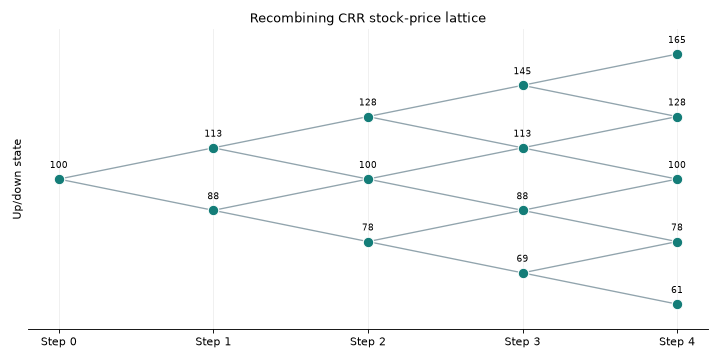
A four-step CRR stock-price lattice. Different paths recombine at shared nodes.
Backward induction
The option value is computed recursively from maturity back to the present. At the terminal nodes, the value is the payoff:
call:
max(S - K, 0)put:
max(K - S, 0)
Then at each earlier node, the continuation value is computed as the discounted expected value under the risk-neutral probabilities:
For American options, the holder may exercise early, so the value is compared against the immediate exercise payoff and the larger of the two is chosen:
This is exactly the logic implemented in the C++ core of the package.
Threshold pruning
crr_price can apply inclusive lower and upper bounds to the stock-price
states. By default, only terminal nodes outside [S_lower, S_upper] are
removed. Earlier nodes remain eligible only if at least one child can reach an
allowed terminal node. With every_step=True, each intermediate node must
also lie inside the band.
Backward induction follows the surviving branches. If both children survive,
the usual risk-neutral expectation is used. If only one child survives, the
remaining transition probability is assigned to it before discounting; a node
with no surviving child has zero value. This is a thresholded lattice valuation
and differs from an unfiltered CRR price. If the root cannot reach any allowed
terminal node, crr_price raises ValueError.
bounded_price = qp.crr_price(
    S0=100.0,
    K=100.0,
    r=0.05,
    sigma=0.20,
    T=1.0,
    N=200,
    q=0.01,
    is_call=True,
    american=True,
    S_lower=80.0,
    S_upper=120.0,
    every_step=True,
)
Assumptions of the CRR model
The CRR model is based on a set of simplifying assumptions:
the underlying follows a discrete binomial process over time
time is divided into a finite number of steps
volatility is constant over the option life
the risk-free rate is constant
the dividend yield or carry rate is constant
there are no arbitrage opportunities in the risk-neutral pricing setup
the tree is recombining, so the number of states remains manageable
These assumptions are standard in introductory option-pricing models and are well suited for educational and benchmark applications.
European vs American options
The package distinguishes between:
European options: exercise only at maturity
American options: exercise at any earlier node
In the pricing function, this is controlled by the american flag:
price = qp.crr_price(
    S0=100.0,
    K=100.0,
    r=0.05,
    sigma=0.20,
    T=1.0,
    N=200,
    q=0.01,
    is_call=True,
    american=False,
)
For a European option, the code follows the standard backward-induction valuation without early exercise checks. For an American option, it compares continuation value against exercise value at each time step.
Black-Scholes benchmark
The package also exposes black_scholes_price, which gives the closed-form
solution to the same problem under the continuous-time geometric Brownian motion
model. This is valuable for two reasons:
it provides a familiar benchmark
it shows how the binomial model approaches continuous-time pricing as
Ngrows
The CRR tree becomes more accurate as the number of steps increases because the lattice approximates the continuous diffusion more finely.
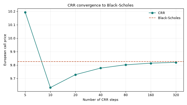
European call prices from the CRR tree approach the Black-Scholes benchmark as the number of steps increases.
How the code implements this
In the C++ core, the process is implemented as a nested loop over time steps and stock states. The numerical sequence is:
compute the terminal payoffs
iterate backwards through time
compute continuation values using risk-neutral probabilities
compare with early exercise when required
return the root node value
In the Python layer, the function only validates user input and then calls the compiled native implementation. This keeps the public interface simple while preserving efficient numerical execution.
This means the model logic is not hidden in Python loops; the expensive calculation runs inside the compiled C++ implementation, while user code remains clean and readable.
Practical interpretation
The CRR model is especially useful for:
teaching option-pricing mechanics
benchmarking numerical methods
approximating option values when closed-form formulas are not available
exploring early-exercise behavior for American options
It is not a complete market model for all exotic derivatives, but it is a clean, transparent framework for vanilla options and for understanding how discrete-time pricing works in practice.